Week 8: Filter-RKHS and revisiting RFF
This week I polished the Filter-RKHS technique from last week. We find this method to be faster and more accurate than the existing ProbSpace. I also revisited the RFF method and found a way of making it faster than the RKHS method through matrix calculations.
Monday :
Discussed the results of the Filter-RKHS method I’d implemented last week with Roger sir. Found out why there appeared to be an offset in some of the graphs. Started working on comparing it with the Probspace method both in terms of time taken and accuracies in the form of average error and a new metric, r2 (r squared) which gives us a value from 0 to 1 based on how well the predicted values fit the ideal curve i.e, if r2 = 1, it’s a perfect fit and vice versa.
Tuesday & Wednesday:
Here is a comprehensive report about the Filter RKHS method, in comparison to Probspace.
Model Used:
X = logistic(0,1)
Y = logistic(1,1)
Z = math.sin(X)+math.tanh(Y)
Some General Observations:
- When calculating P(Z|X,Y=y) we observed a falling-off in the Filtered-RKHS curve after about 6-σ like shown:
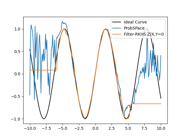
Firstly, while the Probspace curve also falls off after this point, it is not as bad as the RKHS curve(which just flatlines). This skews the r2 calculations (like shown):
Filter-RKHS
Average Error: 0.3696281399936332 r2: 0.18229232980738574
ProbSpace
Average Error: 0.3343384323726664 r2: 0.4050433191928714
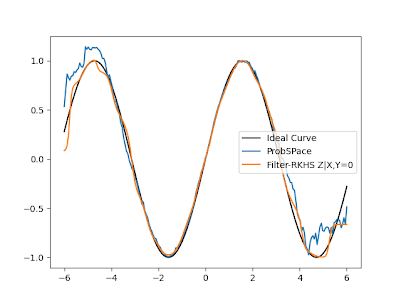
So for this specific calculation (P(Z|X,Y=y)) I will be limiting the X-axis range in (-6,6) going further in my testing.
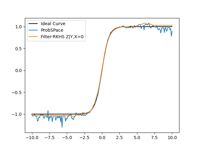
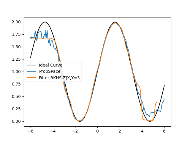
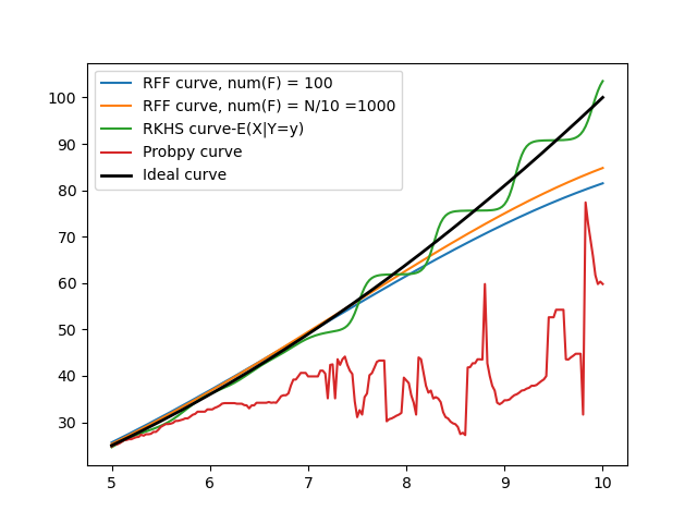
- The Probspace technique is not far off from the Filtered-RKHS when the conditional value is around the mean i.e, when we are conditioning on X = 0 or Y = 0, the accuracies are very close (shown below):
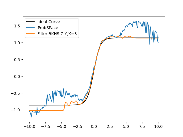
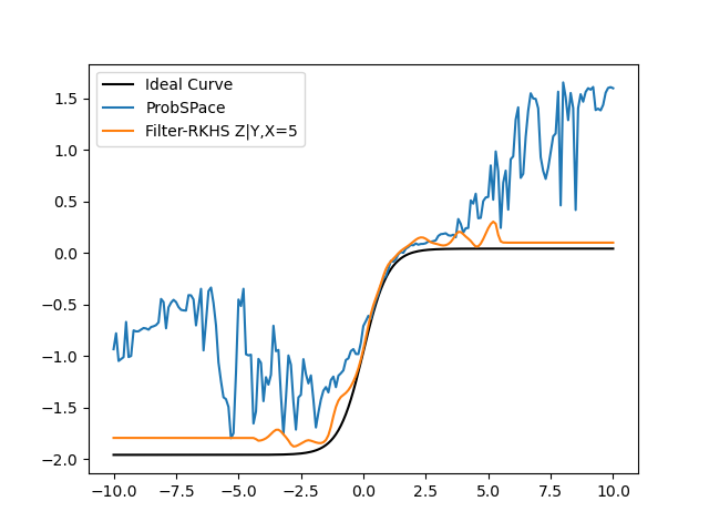
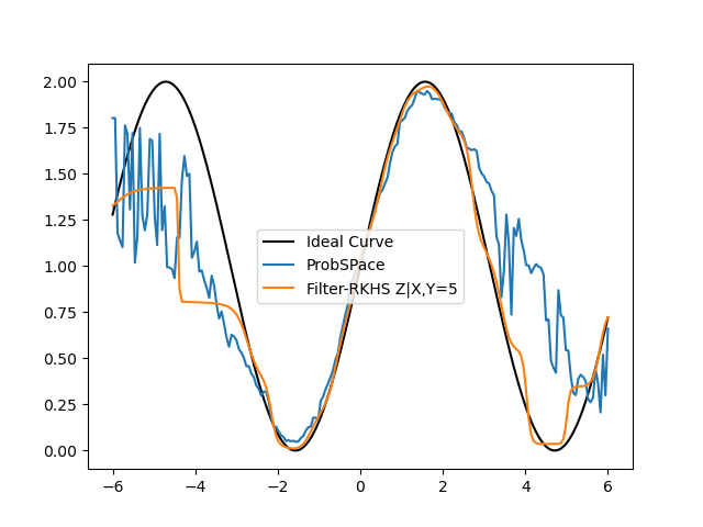
- Where the Filtered RKHS method really shines in comparison is when we are conditioning X and Y on variables farther away from the mean, with lesser data points i.e, say X=3,5 or Y=3,5 for example. This is shown below:
- Here is the Errors Comparison Table:
Time taken:
Thursday & Friday:
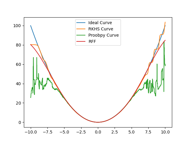
I Revisited the RFF method, after going through all of the theory again and understanding the code implementation, I was able to figure out a way to make it faster than the RKHS method, as it is supposed to be.
Turns out the right method of doing it was through matrix calculations of the kernel approximation matrix, which is different from the iterative approach we have been using for our
RKHS kernel methods. There is an overhead time associated with the RFF method (about 4 seconds) which is required to obtain the approximation matrix. However the time taken to predict is magnitudes lesser than the RKHS method and the ProbSpace method. Here is a comparison of time-taken and errors, for different number of datapoints:
Note: The Overhead time of RFF (4.01 and 4.39 seconds respectively) has not been included in the table above, time taken is measured strictly for prediction.
With this, the RFF method is at a stage that we were initially hopeful about. It produces results comparable to the RKHS method at a faster rate.

Comments
Post a Comment