Week 12: Final Week
These past 12 weeks have flown by so fast! It still feels like yesterday I started working on this project. There were highs and lows but at the end of the day we overcame our obstacles to create something to be proud of. It was a great learning experience and I had fun working with the team.
Monday:
Implemented the prototype of the K decrement algorithm to reduce the number of filter variables in case of shortage of data points upon filtration. Here are some results:
K decrement- condP()
K = 100 rf = 0.8, minmin = 20
dims, datSize, tries, K = 3 1000 1 100
Average R2: JP, UP, PS = 0.67025996194 0.726423475099 0.7434199290171855
K=100 , rf = 0.8, minmin = 5
dims, datSize, tries, K = 3 1000 5 100
Average R2: JP, UP, PS = 0.70784384556 0.87296540935 0.764876980843549
K=100 , rf = 0.8, minmin = 4
dims, datSize, tries, K = 4 1000 1 100
Average R2: JP, UP, PS = 0.70162883565 0.80123074862 0.6089856810665888
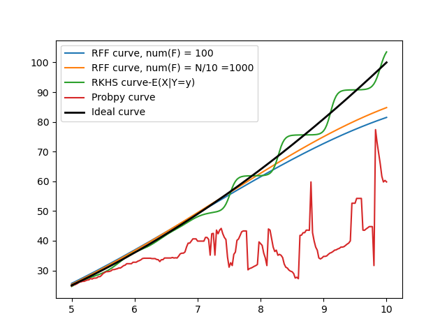
K=100 in condP() function means that we are filtering out all of the variables and then using a single dimensional RKHS to predict the expected value from the obtained data points. As seen it performs surprisingly well, even better than ProbSpace and JPROB.
Tuesday and Wednesday:
I improved UPROB(K=100) for the condE() function to always perform as good as or better than ProbSpace, if not slightly better. Here are some results for datasizes 1000, 10000 and different dimensions::
Datasize : 1000 records
dims, datSize, tries, K, RF = 6 1000 10 100 0.8
Average R2: JP, UP, PS = 0.529763259 0.272241407 0.2835746783497
dims, datSize, tries, K, RF = 5 1000 10 100 0.8
Average R2: JP, UP, PS = 0.7942440087 0.6371377 0.628382190755
dims, datSize, tries, K, RF = 4 1000 10 100 0.8
Average R2: JP, UP, PS = 0.90524824356 0.858100011 0.85786651202
dims, datSize, tries, K, RF = 3 1000 10 100 0.8
Average R2: JP, UP, PS = 0.95138830843 0.923392165 0.92341753255
dims, datSize, tries, K, RF = 2 1000 10 100 0.8
Average R2: JP, UP, PS = 0.97548852478 0.9850602617 0.98458970744
Datasize: 10000 records
dims, datSize, tries, K, RF = 2 10000 3 100 0.8
Average R2: JP, UP, PS = 0.994456329 0.994873499 0.9957236485
dims, datSize, tries, K, RF = 3 10000 3 100 0.8
Average R2: JP, UP, PS = 0.9736031598 0.9606202 0.96381042049
dims, datSize, tries, K, RF = 4 10000 3 100 0.8
Average R2: JP, UP, PS = 0.9541426809 0.94595916 0.9446013055
dims, datSize, tries, K, RF = 5 10000 3 100 0.8
Average R2: JP, UP, PS = 0.8695052963 0.7911628052 0.783551098
dims, datSize, tries, K, RF = 6 10000 3 100 0.8
Average R2: JP, UP, PS = 0.6583874603 0.47835927183 0.486320502
The closeness is because condE(K=100) is essentially just ProbSpace for the most part except for the cases when there are not enough data points, in which case it runs condE(K=80) and so on until enough data points are found.
I've also implemented this K-decrement system universally for condE() so that it works for all K values, not just K = 100.
For example, for a dimension size of 6 (5 conditionals), if the operation condE(K = 80)[ i.e, filtering 4 out of 5 conditional variables ] cannot find enough data points compared to minPoints,
it tries condE(K=60) corresponding to 1 less filtering variable i.e, 3 out of 5.
I've implemented an appropriate K updating algorithm such that it calculates the new K value depending on the number of dimensions and old K value. I've tested this to work for different dimensions, the new K value is always calculated such that it corresponds to one less filter variable, no matter the dimension size. So for dims = 6, it goes 80 -> 60 -> 40 and so on.. and for dims = 4, it goes 100 -> 67 -> 34 and so on.
So we will no longer run into the program crashing due to not enough data points being found
Thursday and Friday:
Prepared and submitted my poster abstract entry as I will be participating in the Poster contest.
I ran a ton of tests and it seems we have achieved what we hoped for regarding the time-taken for execution and accuracy of UPROB(100). He is the general execution times for the three methods:
JPROB - 0.0038 - 0.0048 seconds
UPROB - 0.0017 - 0.0028 seconds
ProbSpace- 0.0010 - 0.0016 seconds
Some observations:
1) The accuracy of UPROB(100) is always equal to or greater than ProbSpace and less than JPROB i.e, accuracy wise: ProbSpace <= UPROB(100) < JPROB
2) UPROB is better than JPROB in both accuracy and time taken when we are dealing with dims>=4 and K~=35 (1 filtered variable).
So in conclusion, while UPROB is always slower than ProbSpace, it is worth using for the better accuracy and faster calculation speeds as compared to JPROB.
Future Plans:
I will be cleaning up the code and implementing an automatic K selection algorithm so that depending on the data size and dimensions, it automatically selects a K value to produce the best results. I will be presenting my achievements during this internship in a meeting scheduled on Aug 24th. I will be preparing a poster for the poster competition and further down the line, I’ll be co-authoring a research paper with Roger sir about the breakthroughs we have made regarding multiple conditioning. If possible, I’ll also evaluate some machine learning algorithms to see how they compare to our techniques in predicting conditional probability.

Comments
Post a Comment