Week 9: Filter-RFF and FPROB
This week I tried extending the filter RKHS method to form a filter RFF method. Unfortunately, filter-RFF does not produce the same quality of results as filter-RKHS. Later, I implemented FPROB or Filter-Probability and tested it against JPROB developed by Roger sir and the existing ProbSpace method.
Monday :
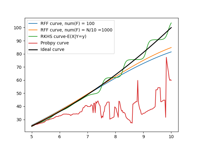
Tried to extend the same principle behind Filter-RKHS to form a Filter-RFF. Here is a comparison between Filter RKHS vs Filter RFF vs ProbSpace:

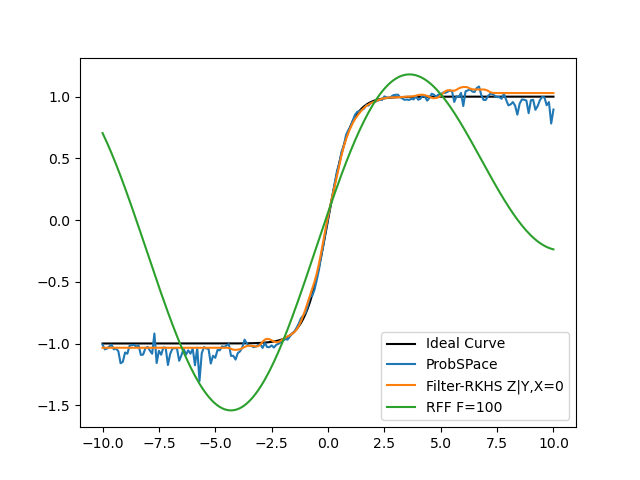
As shown, it does not work very well. Like expected, it is faster than the RKHS variant (shown in table below). But when we are dealing with a small number of datapoints (<1000) anyway after filtration, the RFF method is ineffective. My own conclusion is that it’d be better to use the RKHS method for low data points and the RFF method when we are dealing with massive datasizes and need to speed up calculations.
Tuesday:
During Monday’s discussion with Roger sir, he demonstrated what he had been working on, mainly dealing with JPROB or Joint Probability module which has the capability to perform multiple variable conditioning. My objective is to add the FPROB (the FIlter-RKHS method) to that script so that we can have a comparison between JPROB vs ProbSpace vs FPROB.
And to that effect, I studied the code behind cprobPlot2D.py, cprobPlot3D.py and cprobEval.py. I ran each of them under different conditions and gained an understanding about the overall functionality.
There is also an updated rkhs module, RKHSmod/rkhsMV.py (rkhs-Multi Variate) which as the name implies deals with multiple conditioning. It deals with a multivariate gaussian kernel unlike the regular gaussian kernel we have been using for 2 variables. However, if we are dealing with just 2 variables this module behaves just like the previous RKHSmod/rkhs.py class we’ve been using. So going forward, for all my rkhs methods, I will be using the newer class.
Wednesday & Thursday:
Added my FPROB method to cprobPlot3D.py (here is my code). Here are the 3-D plots for 2 conditional variables ( of the form P(Z|X,Y)) with 1000 data points, 5 tries:

Friday:
Started working on extending FPROB i.e, Suppose we are conditioning on N variables, we might filter N-1 Variables and calculate a single conditional on the remaining variable, or like Roger sir suggested, we could try filtering all N of the variables and try plotting the remaining data points using a univariate kernel. It would be interesting to compare these results. Another interesting metric to find would be what % of variables do we filter and perform JPROB on the rest to obtain the best results.
Upcoming week plans:
Create a new module, UPROB, that has the same functionalities as rkhsMV.py but also encompasses JPROB and FPROB, taking a metric k such that we filter k (or k%) of N variables and perform JPROB on the rest. So at k=0, it is just going to be JPROB and k= N-1 would be the 2D Filter-RKHS method I’m currently using.

Comments
Post a Comment