Week 7: Getting started with Filter-RKHS
This week I revisited the RKHS method to confirm that we are on the right track and got started with implementation of the Filtered-RKHS method. Here is a day-wise summary of my progress throughout the week:
Monday & Tuesday:
Analysed the RFF code to reduce the time taken for calculations. Implemented an RFF calculation method according to the formula:

As described in this article where z(x)T z(y) is the equivalent calculation to k(x,y), the basic kernel function. The kernel techniques we employ use an iterative approach instead being performed through matrix operations. As a result of this, it involves calling the k(x,y) function repeatedly over the length of the dataset to produce results. I could not figure out how replacing the RFF calculations instead of RKHS kernel calculations would speed up the calculations. If anything, it is going to be slower because while the k(x,y) function is a straightforward calculation, the RFF method iterates over R random selected features as the formula shown above indicates. I must have gone wrong in my calculations somewhere or misunderstood some concepts. I will be revisiting this method again to figure it out after discussion with Roger Sir.
Wednesday:
To reinforce that the RKHS method we have been using so far is reliable, I tested it with different models other than the Y= X2 model which we have been using for weeks now. Here are some of those results
 |
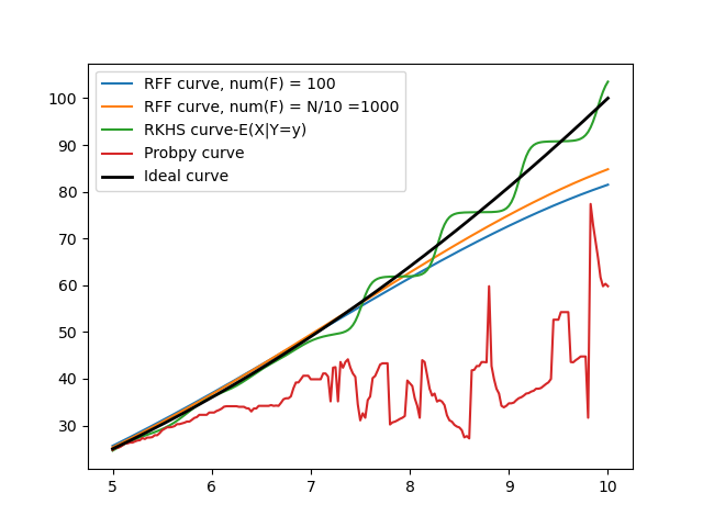
| Y = sinh(X) |
 |
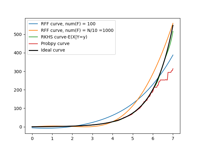
| Y = exp(X) |
 |
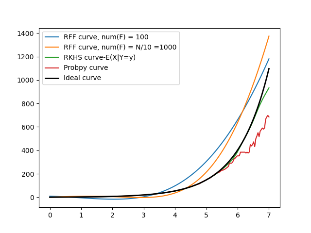
| Y = tanh(X) |
 |
| Y = tanh(X) + X2 |
Thursday & Friday:
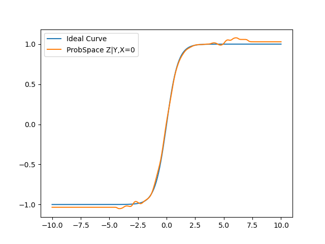
The ProbSpace Z|Y,X=0 is the curve where data points have been filtered through the Probspace method and then the RKHS method has been applied to calculate P(Z|Y) on it.
As seen, the curve resembles a tanh() curve, which is what Z is when the influence of X has been removed.
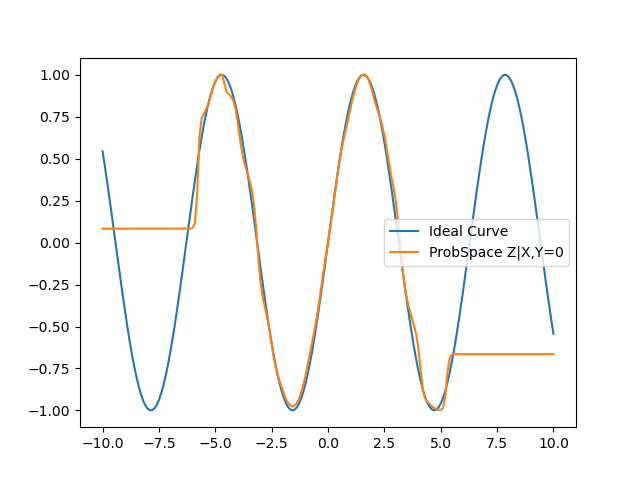
Similarly, in this curve we are calculating P(Z|X,Y=0) i.e, we filter based on value of Y and then calculate P(Z|Y). The obtained curve resembles a sin() curve, which is nothing but Z with the influence of Y removed.
These results are excellent, however the obtained curves are only so accurate because of the high availability of data points i.e, since X=0 and Y=0 are around the mean of the dataset, we were able to filter a relatively large amount of datapoints in close vicinity to 0. However, as we condition on points farther away from the mean, X = 5 or Y = 3 for example, there are fewer data points available, even when the σ value is increased. This leads to poorer results. The graphs and Average Error table is shown below:


Comments
Post a Comment